


Who: Assembling the Team and Starting Production
“Coming together is a beginning. Keeping together is progress. Working together is success.” - Henry Ford
Series Overview
The FAIR™ Ontology and open SIPmath™ standard are complementary methodologies for managing risk and communicating uncertainty respectively. Combining FAIR and SIPmath provides a revolutionary way to link risk models with revenue models of various sorts to gain an enterprise-wide view of risk/return tradeoffs.
Read the blog post series on FAIR meets SIPmath
 Coming Together
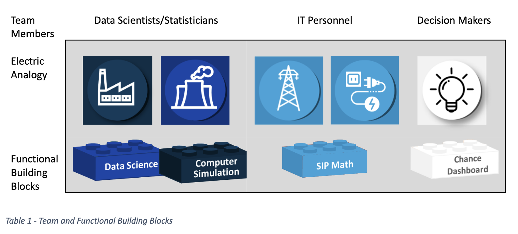
Traditionally, quantitative risk modeling has been done by highly technical data scientists and statisticians. They would typically create monolithic computer simulations from data and expert opinion. The results were often transmitted to the decision makers in the form of written or power point reports containing technical jargon that triggered Post Traumatic Statistics Disorder (PTSD). The FAIR-SIPmath approach connects your existing Data Scientists, IT Personnel, and Decision Makers through SIP Libraries that convey uncertain risks and opportunities as auditable data.
SIP Libraries may be created in one part of the organization using one computational platform by people with a high level of statistical training, then stored in another part of the organization, and finally assembled into models and dashboards anywhere else on diverse platforms to be used by decision makers regardless of statistical training. This is analogous to electricity being created in a power plant, sent across transmission lines, and ultimately used in a light bulb as shown in Table 1.
Keeping Together
Your firm’s data scientists and statisticians should have little trouble creating SIP Libraries from their current models using R, Python, or virtually any other computational platform. The IT Personnel can easily handle the JSON or CSV format of the SIP Libraries, or if needed translate the data into some other text-based format. The Decision Makers can forget most of what they learned in their statistics classes, because the laws of probability are baked into the SIP Libraries. This means that they may be added, subtracted, or even multiplied just like numbers, as shown in Figure 5. In the FAIR-SIPmath approach the team is kept together through the continual development of small prototypes of various aspects of the system, which may be scaled up and aggregated into a full system. This is very different from planning a large system that never seems to work as planned.
Working Together
Once the production environment is set up, unlike a monolithic system, modules may be swapped in or out and improved incrementally. This enhances the maintainability and evolution of the system.
Business Scenarios
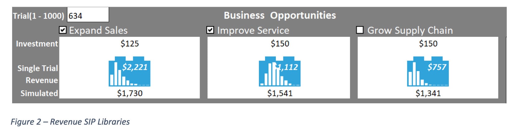
We will demonstrate the production environment in terms of a firm that wishes to grow to the next level by means of three investments. It may Expand Sales, Improve Service, Grow its Supply Chain, or any combination thereof. However, management is not certain about the revenue associated with any of these opportunities.
Revenues
To quantify the uncertainty for each opportunity the analysts have created revenue simulation models that generate 1,000 simulated trials. There are no restrictions on the platform or type of revenue simulations used. For example, one might be a Monte Carlo simulation in Excel, one an Agent Based simulation in Python, and the third the output of a calculation in R. What is critical is that the outputs of each model are stored in an associated SIP Library as shown in Figure 2. For this proof-of-concept example you may think of each library as an array of 1,000 simulation trials, of which trial 634 has been selected for viewing. The bar graph on each building block is simply the histogram of values in that library, which is shown along with the simulated average value below the block. In the downloadable model, a check box allows selection of each of the three opportunities into the investment portfolio.
Risks
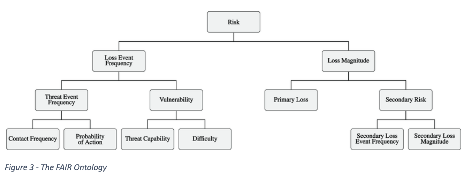
Each business opportunity introduces its own information risk, and each risk offers the option of investing in a control to reduce that risk. We will model this using a simple version of the FAIR Ontology.
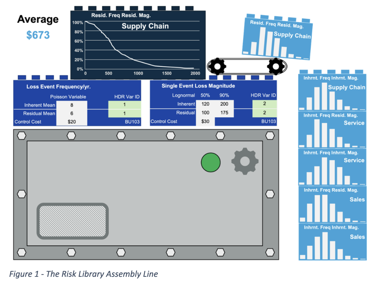
Loss Event Frequency
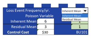 For the business unit displayed, the Analytics team has modeled Loss Events with Poisson variables. They have determined an Inherent Frequency with an average of 6 events per year. If the firm institutes a $30k control, selected by a pull-down menu, the average can be reduced to a Residual of 3 per year. The block shown is for the Sales Expansion opportunity and there are similar blocks for the other two opportunities.
Loss Magnitude
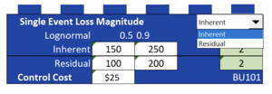 For this business opportunity the analytics team models Loss Magnitude as a Lognormal variable. The Inherent Magnitude has a 50th Percentile of a loss of $150k and a 90th Percentile of $250k. A $25k control will reduce these to $100k and $200k respectively.
Computer Simulation
SIP generation is usually performed by Monte Carlo simulation but can also be done using more complex methods. In the FAIR Ontology, simulating the risk involves simulating a number of Loss Events as one random value and then summing that number of independent Loss Magnitudes. For example, suppose on one simulation trial, three Loss Events were generated. Then three independent random Loss Magnitudes would need to be generated and summed. If on the next trial, there were 15 Loss Events then 15 Loss Magnitudes would need to be summed. This can be very time consuming to simulate, but a recent breakthrough involving the Metalog Distribution provides an analytical solution to summing independent Loss Magnitudes from almost any continuous probability distribution.
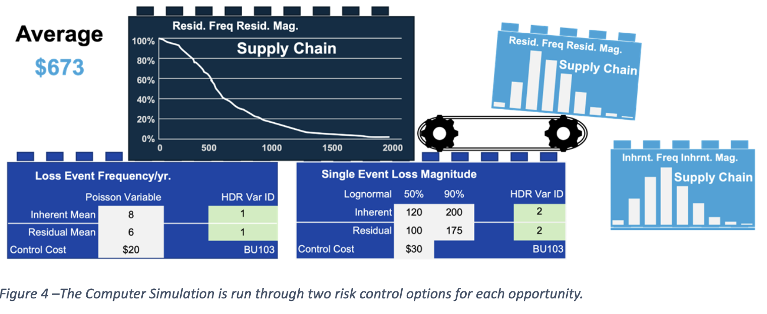
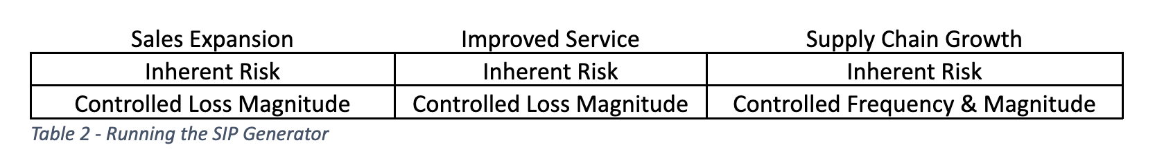
Figure 4 displays the Computer Simulation, two Data Science blocks and resulting SIP Libraries for the Supply Chain opportunity as it cycles through the inherent and residual risk. Table 2 below shows the combinations for all six Risk SIP Libraries considered for the investment decision.
http://www.metalogdistributions.com/images/Metalogs_and_the_Sum_of_Lognormals_in_Closed_Form.pdf
The six libraries generated are displayed in Figure 1 at the top of this article. These are combined with the three Revenue libraries and associated cost numbers to create all possible portfolios of investments as shown below.
Assembling the Libraries
How many distinct combinations of investments are there? There are three choices for each of the opportunities, that is pass on it, take it with the Inherent risk, or pay for the Residual risk with a control. So, altogether for three opportunities that makes 33 = 27. Will we need to run 27 simulations, one for each possibility? Not with the FAIR-SIPmath approach. Instead, we will combine the nine SIP Libraries simulated above. Going from 27 down to 9 might not seem like a lot. But if there had been 10 business opportunities, each with three options, the number of simulations would have grown exponentially to 310 = 59,049 simulations. This is reduced to only 30 with the building block approach. The SIP Libraries required for each investment can now simply be assembled as needed for each of the 27 investment opportunities. The assembly of the block for Sales with Inherent Risk and Service with controlled risk is shown in Figure 5. Remember that each block contains 1,000 trials. Trial 634 is displayed. Note that each of the two business opportunities is assembled from two previously calculated SIP Libraries to form a model of that opportunity (small white blocks on the left of Figure 5). Then, due to the modularity of SIPmath, these two blocks may be further combined to create the portfolio comprised of those two business units.
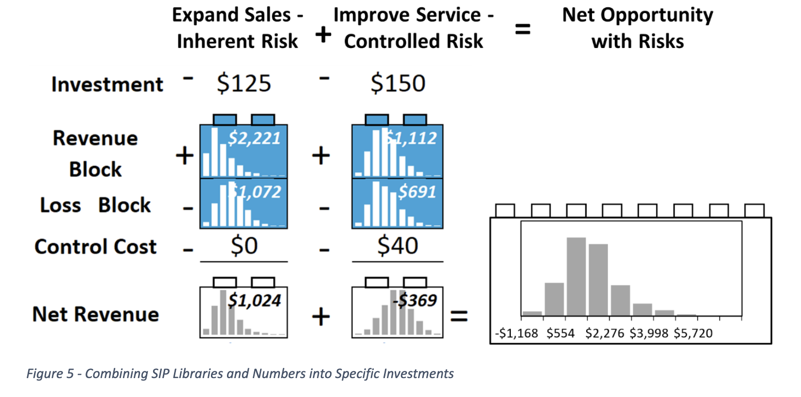
Note that SIP Libraries and numbers can be combined with ordinary arithmetic operators. Also note that the Risk SIP Libraries, investments, and control costs enter the equations with minus signs because they represent money going out.
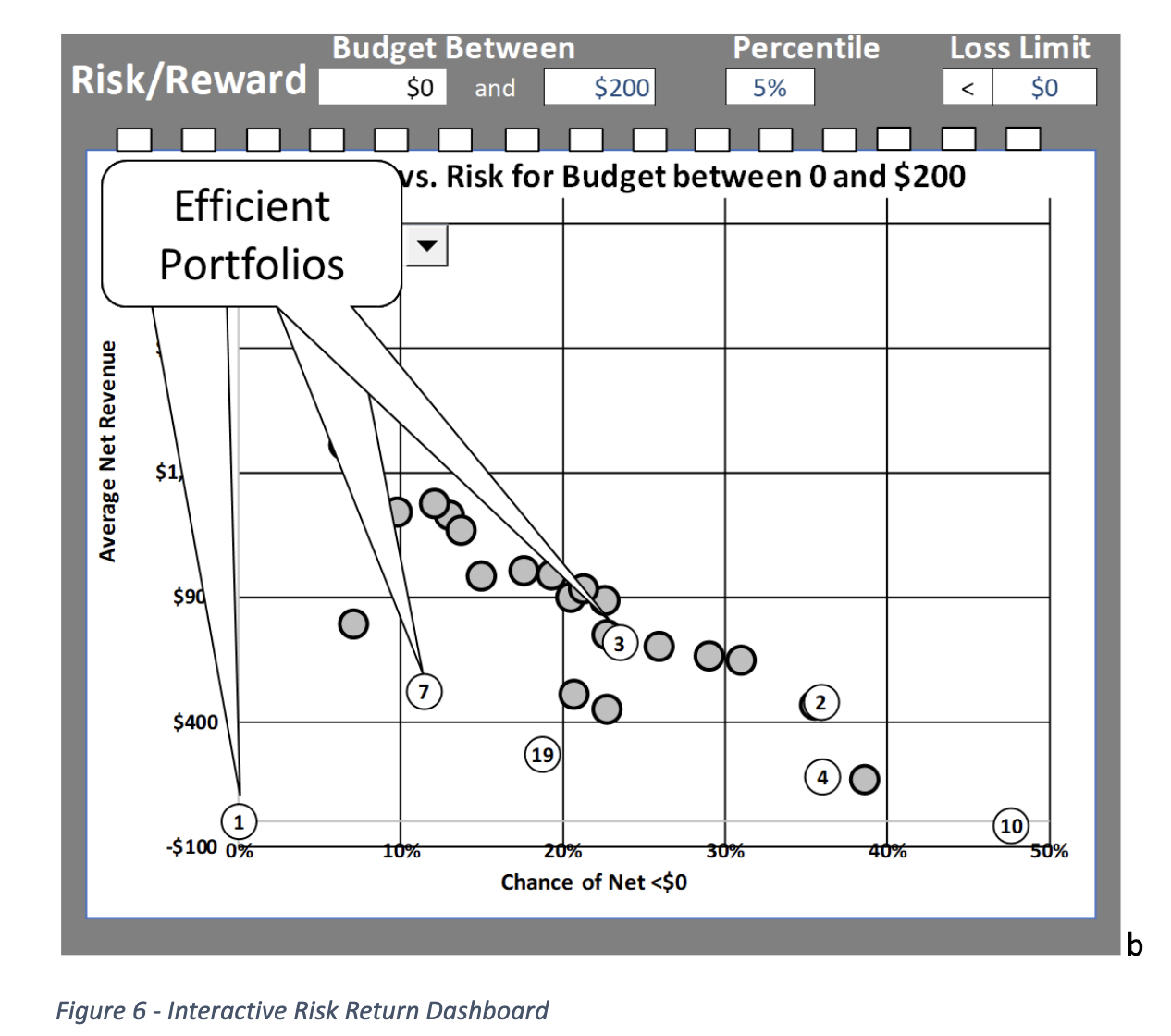
In the next installment we will show how the models described here and in part 1 may be used to automatically generate SIP Libraries for all 27 investment options so their risks and expected revenues may be compared on the same graph. The interactive dashboard shown in figure 6 allows decision-makers to experiment with investment budget and loss limits, and instantly observe the risk/reward tradeoffs. For the budget shown, portfolios 1, 2, 3, 4, 7, and 19 are available, and 1, 7, and 3 are on an efficient risk/opportunity tradeoff curve. That is, all other portfolios offer both more risk and less opportunity than 1, 7, or 3.
About the Authors
John Button
Gartner Risk Advisor. Managing editor of several publications including FAIR-CAM Control Physiology, Cultural Calamity, The Tao of Risk Management, and The Drone Age.
Dr. Sam Savage
Author of The Flaw of Averages – Why we Underestimate Risk in the Face of Uncertainty and Chancification – Fixing the Flaw of Averages, Executive Director – ProbabilityManagement.org, Adjunct Faculty – Stanford University Dept. of Civil & Environmental Engineering.
Eng-wee Yeo
Principal, Technology Risk Modeling & Methodology at Kaiser Permanente. He is responsible for modeling, simulating and assessing non-financial technology risks to support decision making.
The FAIR Institute welcomes submissions to our blog from our members. Please contact us.


.jpeg)
.png)
.png)