 Search “return on security investment” (ROSI) or any of its related terms and you will see a consensus on a calculation that compares your reduced risk (or monetary loss reduction) to the cost of your mitigation.
There are risk mitigations that are quick and cost-effective (e.g., software patch, an application configuration, disabling a service, etc.); however, others like those managed by an Enterprise PMO or involving professional services may span several budget years and require additional financing.
The consensus ROSI is perfectly suitable for making decisions on the former quick-hit use cases but is insufficient as an aid to providing valuable context to decision-makers weighing the alternatives of more complex projects and programs that have mitigation potential.
 Author Caleb Stogner is Senior Information Risk Engineer, GRC, for Equinix and a FAIR Institute member. We welcome contributions to the FAIR Institute blog. Contact us.
As FAIR™ practitioners we understand the value of better models and the dangers of relying heavily on weak assumptions. This guide demonstrates how a common financial valuation method, discounted cash flow (DCF) analysis, can be used alongside our FAIR assessments to produce greater quality in our cost comparisons against risk mitigation alternatives.
Limitations of Security ROI (ROSI)
My challenge to the consensus ROSI calculations mentioned above is that as risk analysts, there are some decisions we support with cost-benefit analyses where the upfront costs do not take place within a single year. Consider a multi-year implementation project intended to mitigate a risk assessed at $150K ALE, where:
•. Labor and professional services to stand up a new capability costs $100,000 in the first year, $50,000 in year 2, and $20,000 each year thereafter as a subscription cost.
•. The capability does not begin reducing risk until after year 2 but is expected to reduce risk by 70%.
This example is summarized in Table 1 below:
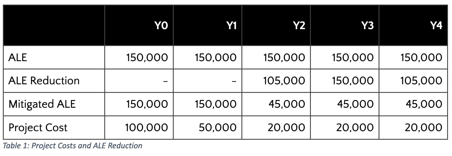
How would we present ROSI under the consensus definition for the above example? No single year captures the full picture. Only when combining the multi-year costs can we begin to effectively compare these cash outflows and risk reduction overtime.
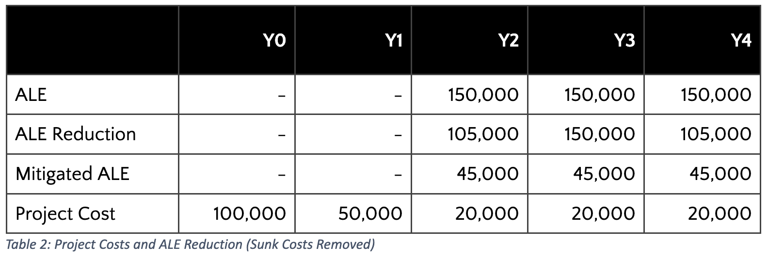
Before totaling these amounts, consider whether any of the amounts shown are sunk costs that should be excluded. Our choice of whether to proceed with the project (i.e., mitigate the risk) has no impact on ALE in years 1 and 2. As sunk costs, those two years’ ALE should not factor into our calculation
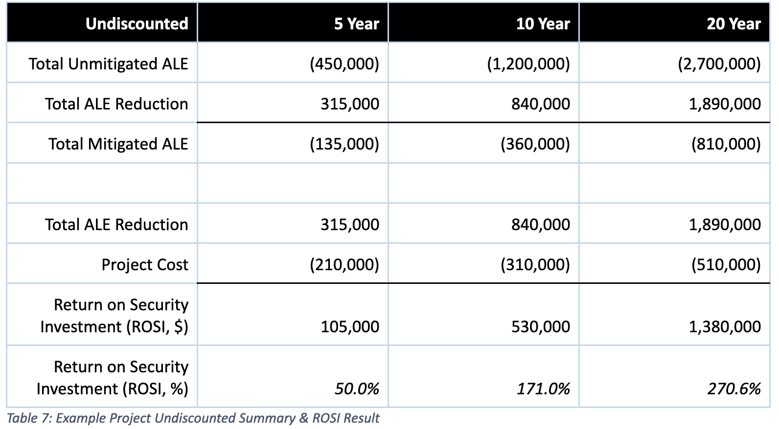
Adding the five years together allows us to calculate a new multi-year ROSI:
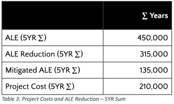
Here, we arrive at a positive ROSI [50% = (315K - 210K) / 210K] under the consensus model. Now, many readers will already recognize that if we chose to forecast timelines greater than 5 years, the ROSI would continue to grow more favorably. To address this objectively and consistently with how organizations tend to evaluate other capital budgeting decisions, we ought to consider how DCF can accompany FAIR analysis for cost-benefit decisions.
![]() Join the FAIR Community. Network with your peers and thought leaders at the leading edge of the risk management profession, the FAIR Institute.
Join the FAIR Community. Network with your peers and thought leaders at the leading edge of the risk management profession, the FAIR Institute.
Brief Discounted Cash Flow (DCF) Primer
DCF enables organizations to compare potential project alternatives and to make decisions based on profitability over time. DCF is based on an assumption that an organization’s use of each dollar has an opportunity cost. Potential “opportunities'' for these dollars include revenue-generating operations, capital projects, and investing the money elsewhere.
This opportunity cost is normally reflected in DCF as the organization’s growth rate or cost of capital, but arriving at this value is outside the scope of this blog post. For our purposes, we will refer to this rate by its more descriptive name – the required rate of return. Think of the required rate of return similarly to how we use risk tolerance in our programs. It is a meaningful, but arbitrary selection that helps aid in decision making based on expectations of what amount of risk (or return) is acceptable to the business.
Integral to DCF is a concept called the “time value of money”. If given a choice to receive $1,000 today or $1,100 next year, which option should you take? The answer depends on what you expect to be able to do with that additional year. If you can grow your money by greater than 10% within a year, you would be better off with taking the $1,000 today; whereas if your prospects were lower than 10%, waiting to receive the $1,100 at the end of one year would be to your advantage.
DCF techniques enable analysts to weigh these types of decisions efficiently and over more complex cash flow structures. Before continuing I want to briefly call attention to the way I labeled each year in the tables above – beginning with Y0 (Year 0) instead of Y1 (Year 1).
How we will incorporate DCF into our examples is by using Present Value (PV), which measures the equivalent value in today’s dollars (Y0 dollars) rather than future year’s dollars. Another way of thinking of the year labels is that Y0 represents today, Y1 is one year from now, Y2 is two years from now, and so on.
The math behind DCF is not difficult and is made even simpler thanks to Excel formulas which will be covered soon for practical application. If you already know the fundamentals of DCF or only care to see how to calculate it within Excel practically – skip down to section “Where DCF and FAIR Align”. If you wish to see some theory behind this concept, continue reading.
Let’s hone in Y2 in the table above. We want to measure the $105,000 ALE reduction and the $20,000 annual maintenance cost in today’s (Y0) dollars. For demonstration purposes we will use a 15% required rate of return. Since these occur in the future, we need to calculate the PV of these amounts in order to determine what their value is in today’s dollars assuming a 15% required rate of return. Below are two representations of how to calculate these amounts:
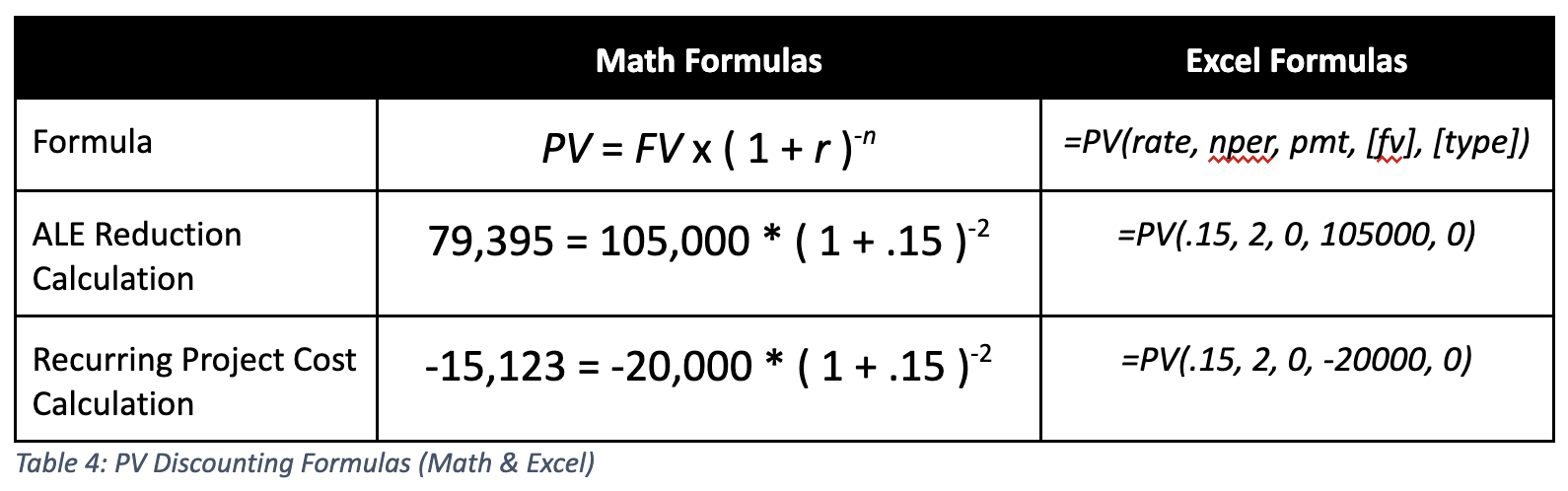
Math Formulas
Where n is the number of periods considered, r is the required rate of return, and FV is the future value (i.e., value in Y2 of our risk reduction and cost of the annual maintenance). My recommendation for new readers is to leverage Excel’s formula libraries.
Excel Formulas
When using this formula, set pmt to 0 which involves annuities, which we won’t need. When using Excel, be sure that your costs are reflected as negative values and that benefits are formatted as positive numbers.
Where FAIR and DCF Align
The great news is – you do not need to do year-by-year calculations like those above! You can utilize other formulas within Excel to handle most of the complexities and focus on getting to the metrics you would use for comparisons and decision making – Net Present Value (NPV) and Internal Rate of Return (IRR).
In our role as FAIR analysts, we are no strangers to assessing decision alternatives quantitatively. In fact, our assessments often compare annualized expected loss to the costs of risk mitigation or control implementations. Seldom discussed in our field is how to represent those costs when the mitigations or implementation costs occur in larger project structures that span multiple years, as explored in the initial example.
NPV and IRR are metrics used to represent a project’s returns based on its future expected cash flows. Fortunately, both can be easily calculated in out-of-the-box Excel formulas (each is hyperlinked to Microsoft’s documentation page):
=NPV(rate,value1,[value2],...)
For the IRR formula, values must contain an array of positive and negative amounts (remember your costs must be negative – net your costs and benefits if both occur in the same period). NPV requires a required rate of return at the rate and then can accept an array of values or individual values separated by commas.
What are these metrics calculating? Well in the above PV formulas, we calculated the PV of one year’s benefit (the risk reduction) and cost. NPV would calculate the PV of benefits and costs in each year (net together, so each year has one value) and sum them for a total dollar amount above our required rate of return. Let’s see what that looks like for our example:
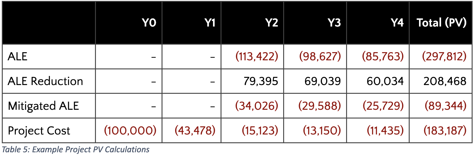
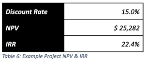
Remember, in this example a 15% required rate of return was selected. To reach the NPV, total all relevant benefits (ALE reduction in our case at $208,468) and subtract all relevant costs (Project Costs at $183,187). Since the NPV of $25,282 is a positive number, the project's rate of return is greater than the required rate of return. IRR calculates something similar – the internal rate of return where NPV breaks even. In the case of this example, IRR is 22.4%. When IRR and the required rate of return (r) are equal, NPV is $0. If the required rate of return was set to 25%, the NPV would be negative, and the IRR would remain unchanged at 22.4%.
One final comment on choosing between IRR and NPV for your analyses. Comparing alternatives using IRR is often more convenient since a required rate of return input is not needed. Keep the end in mind, and if you are simply prioritizing alternatives, the rates output as IRRs may be sufficient for your analysis, but if you are needing dollar values – acquiring the appropriate required rate of return input for an NPV analysis may be worth the additional time.
To recap, when NPV is positive or when IRR is greater than your required rate of return (and these always coincide), we can conclude from this example:
•. The benefits (i.e. reduced risk) of the project are greater than the cost of the project overall.
•. Even if the organization had an investment that would guarantee the required rate of return of 15% (i.e., a bond or a business venture), we would still be better off proceeding with the project because it is expected to benefit the organization at a rate of 22.4%.
For further reading and examples of how to use these techniques, consider additional reading on discounted cash flow analysis, IRR, NPV, and capital budgeting. Some good resources for each are linked at the bottom of this blog post.
Where to Stop?
The challenge in applying discounting is determining how far into the future you forecast cash inflows and outflows. In other words, when have you considered enough years and when can you stop? On an undiscounted basis, the difference between a 5YR, 10YR, and 20YR time horizon is significant:
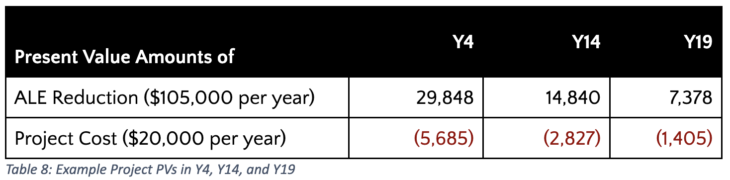
Discounting helps address these concerns by weighting each subsequent year less as you approach the end of the analysis. In the final few years of each of the time horizons shown above, the original ALE reduction of $105,000 each year and recurring project cost of $20,000 are reduced to:
Now for the discounted summary:
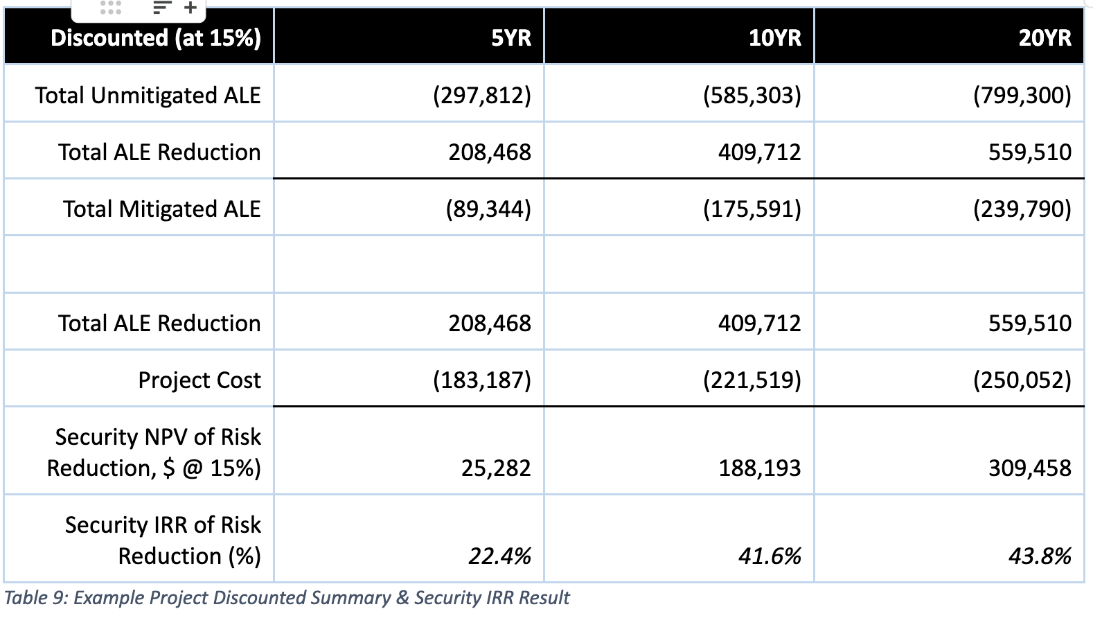
The example’s results indicate the IRR on the project seems to converge somewhere around the 42 - 44% mark. Though every project is unique, if presenting the IRRs only there is little reason to forecast beyond 10 years in this example. Since PV calculations in DCF are inherently weighting each year’s benefits and costs, there is a range somewhere in the 3 – 15 year timeframe that is likely going to meet most of your needs if performing DCF within your assessments. Assessments with time horizons greater than 20 years should be rare, and as previously stated, assessments with two-year timeframes or less are not likely to be worth full DCF treatment.
Parting Thoughts
Following this methodology is tedious, even if you are familiar with both FAIR and DCF, and I would not recommend applying it broadly to every assessment and cost-benefit decision you support in your organization. Always align the level of effort in your analysis to the complexity and significance of the decision you intend to support.
DCF is yet another technique we can add to our risk programs that can offer value when applied to complex cost-benefit decisions that pertain to risk. I recommend including DCF in those rare circumstances where large multi-year projects must be evaluated and compared based on their risk reduction potential. Consider some of the possible use cases below:
•. Compare complex long-term projects' risk mitigation potential over time:
º Select the project with the higher IRR/NPV
•. Compare a risk mitigation project or control implementation with an investment project:
º. Compare the risk mitigation IRR against a traditional IRR but be prepared to defend the noncash expected losses inherent in your FAIR modeling
•. Compare cost structures of risk mitigation or control implementation projects:
º. Look at pricing models of mitigation projects including SaaS vs. on-premise, different SOWs during bidding, and select what is most advantageous for your business.
For decisions that can be mitigated within one or two years, I would not expect these techniques to be worth the additional analysis beyond an undiscounted cost-benefit analysis.
Further Reading
For every linked resource here, there are many others that capture the concepts equally well. Many of these also cover the additional assumptions and drawbacks inherent to the underlying math that would occupy too much real estate to include within the post. Consider the following articles for additional examples and explanation:
- Time Value of Money
- Discounted Cash Flows
- Net Present Value
- Internal Rate of Return
- Capital Budgeting
![]() Join the FAIR Community. Network with your peers and thought leaders at the leading edge of the risk management profession, the FAIR Institute.
Join the FAIR Community. Network with your peers and thought leaders at the leading edge of the risk management profession, the FAIR Institute.
.jpeg)
.png)
.png)